Upon Matrix and Graph Representations of Factor Graphs

MotivationPermalink

• Understand better the connections between matrices and graphs in previous works; Recap details.
  • Factor Graphs for Robot Perception
• Have a glance at advances in the intersection of graph theory and SLAM
  • Reliable Graphs for SLAM, IJRR 2019
  • Cramér–Rao Bounds and Optimal Design Metrics for Pose-Graph SLAM, TRO 2021

Factor Graph and its Information MatrixPermalink

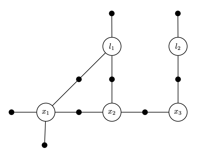
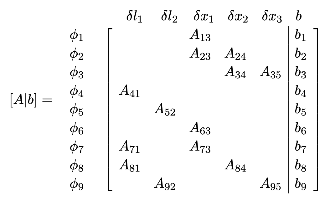
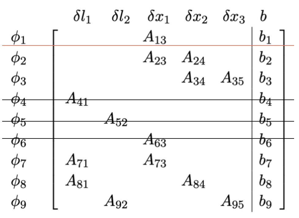
We start with revisiting a factor graph and its corresponding Jacobian

• Each factor corresponds to several rows. It is a measurement.
• Each variable corresponds to several columns. It is a state to be estimated.

So we have a factor graph, and its corresponding linear system $Ax = b$.

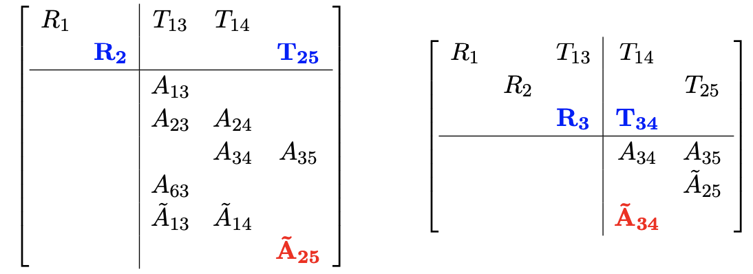
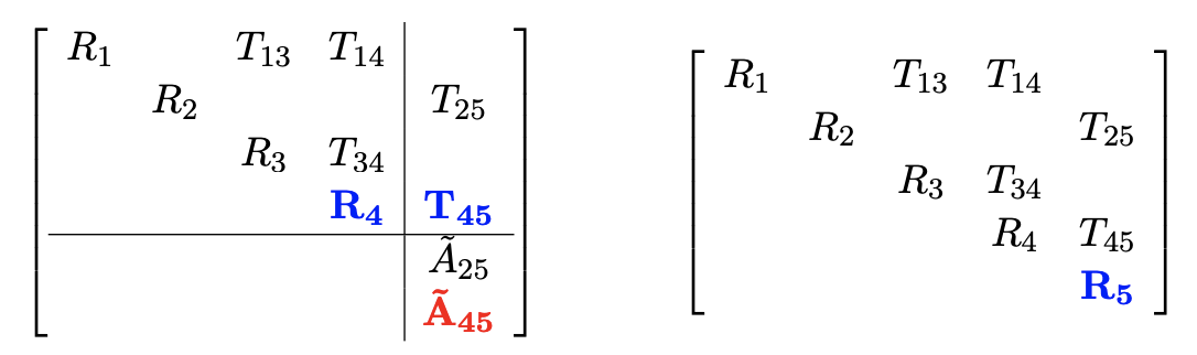
Variable elimination and matrix factorizationPermalink

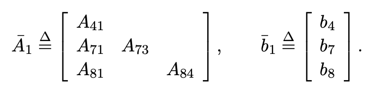
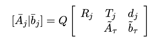
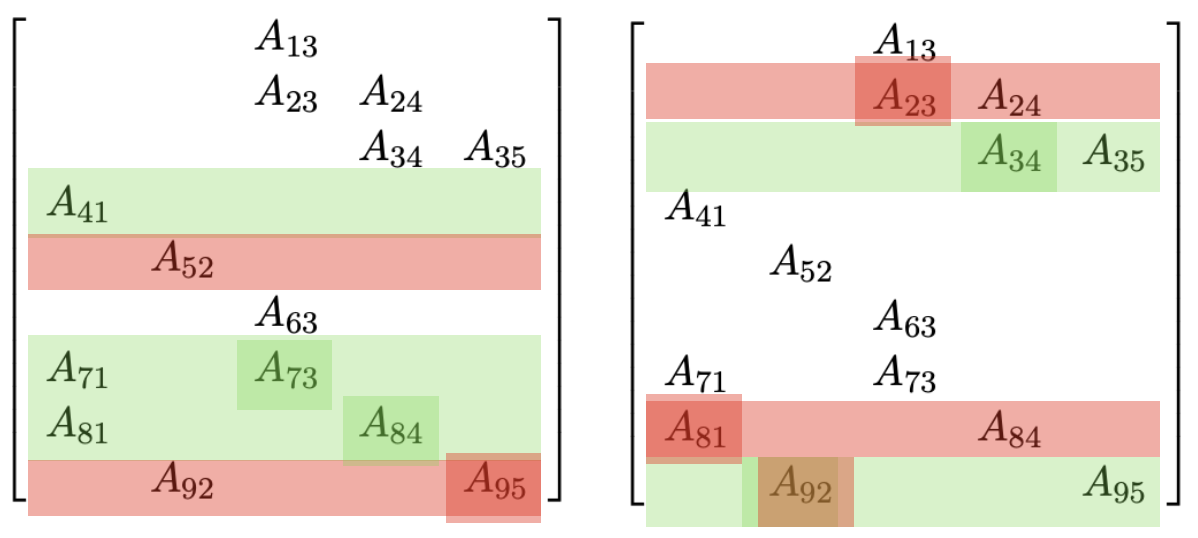
In large sparse SLAM setups, we usually factorize A with QR. Partial QR is iteratively applied to submatrices, with permutation (?).

• Factorization is variable elimination in a graph
• The spirit is like ‘an undirected graph to a DAG’

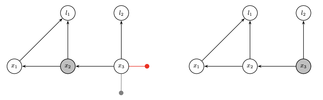
• Factorization is partial QR in a matrix
• Use Householder reflections or Givens rotations

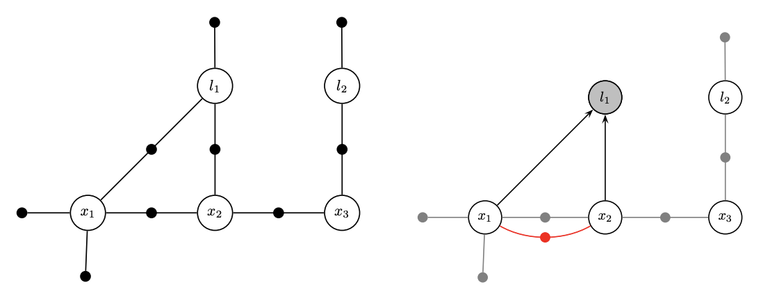
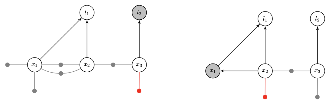
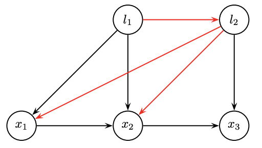
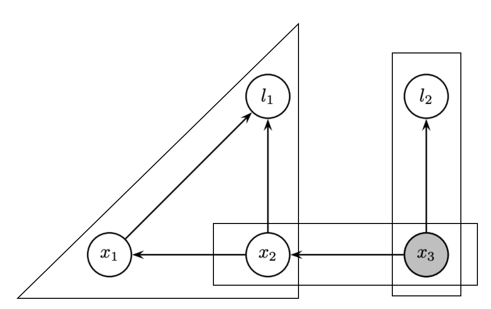
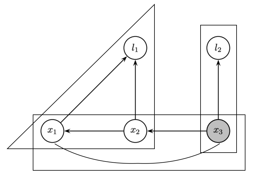
Variable elimination orderingPermalink

The ordering in elimination matters. A bad order results in fill-in and leads to a dense matrix to solve.

• Topologically densely connected

• We prefer smaller degrees in order

  

• Degrees:
  • l1=1, l2=1; x1=2; x2=3, x3=2.

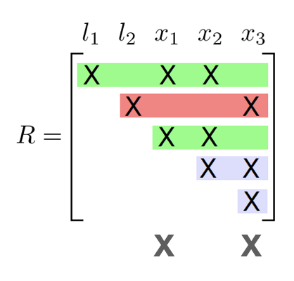
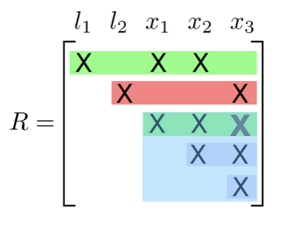
• Computationally dense

  

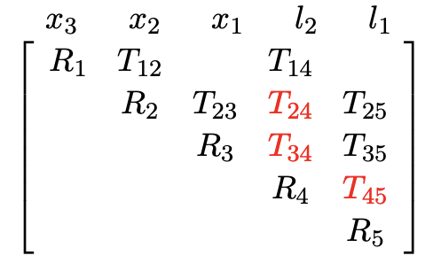
• We prefer fewer entries in the rows during QR
  • Direct order: 2 fill-in, then 1 fill-in
  • Inverse order: 2 fill-in, then 3 fill-in

  

Heuristics for reorderingPermalink

• Reorder according to degrees: COLAMD

  [TODO] https://citeseerx.ist.psu.edu/viewdoc/download?doi=10.1.1.124.1109&rep=rep1&type=pdf

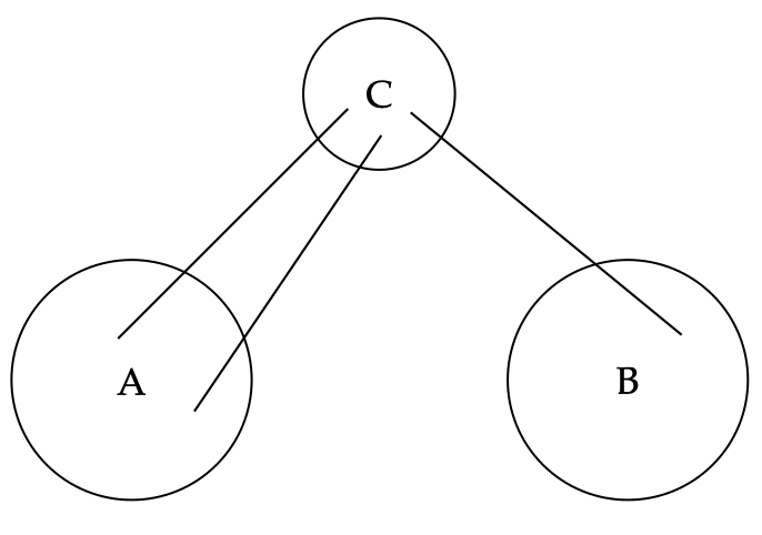
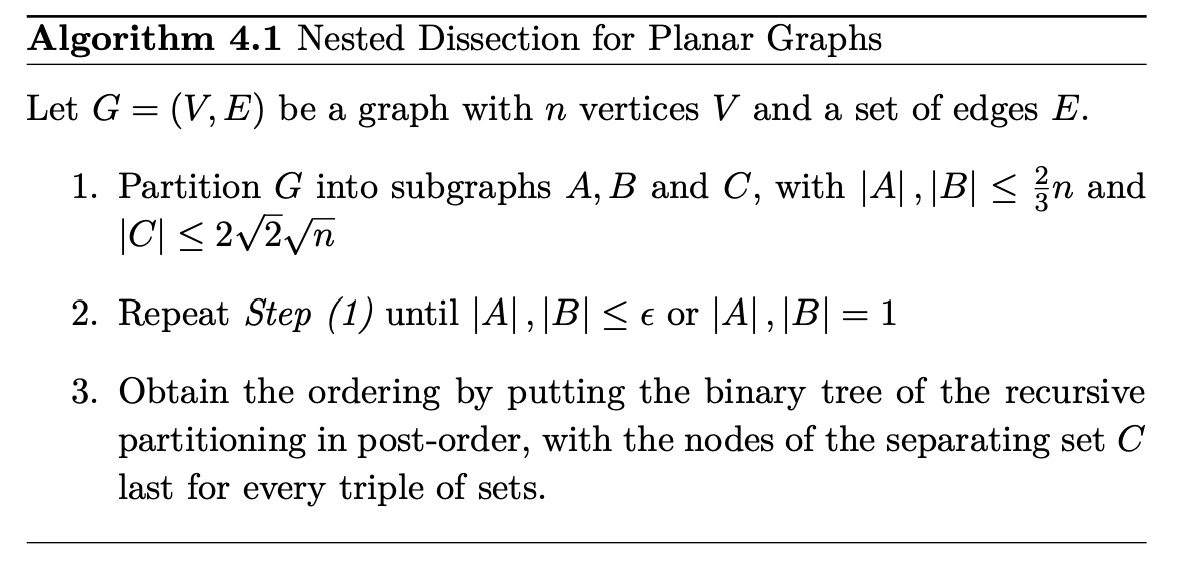
• Graph partitioning: METIS

• A graph can be somehow partitioned into

  

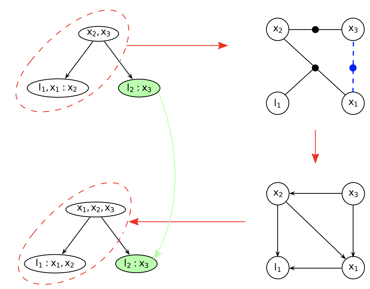
Incremental update and the clique treePermalink

Fact 1

• Variable elimination results in not only a DAG but also a chordal graph (PGM Theorem 9.8)
  • A chordal graph is a triangulated graph

  

Fact 2

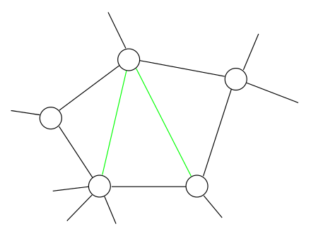
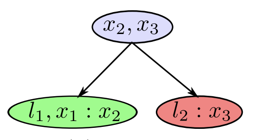
• We can form a clique graph from a graph, by connecting max-cliques

  

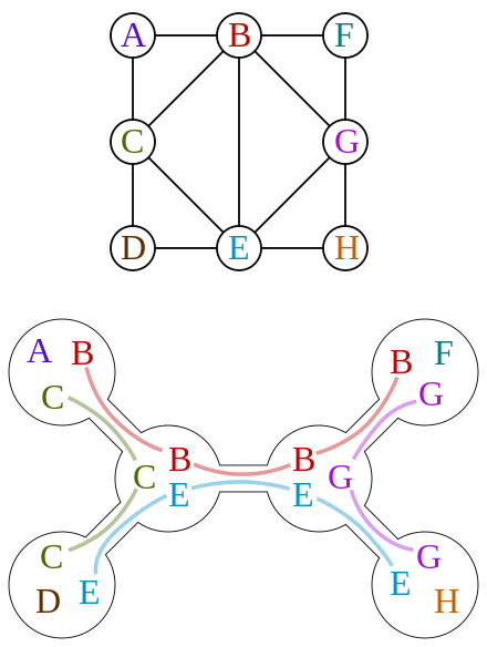
Fact 3

• A clique graph is a clique tree in a chordal graph

• Trees are good for elimination or factorization esp. when the cliques are small

• A clique tree depicts the global structure

  

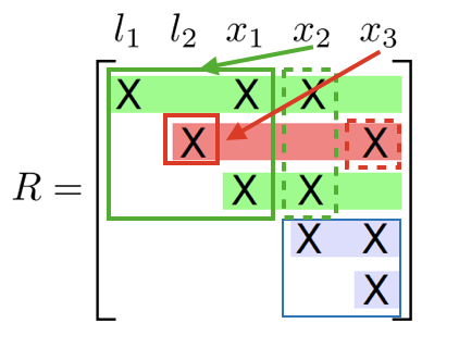
• Each clique depicts local distributions

  

• In a clique is a dense upper triangular matrix after reducing the separator column

  

Incremental update

• Identify the path from the root that contains the variables
• Redo the variable elimination locally to update the clique structure
  • Givens rotation locally

  

  

SummaryPermalink

Up to now, we know the connection between

• Matrix factorization (QR decomposition, reordering rows, locally dense triangles)
• and graph topology manipulation (undirected to DAG, factor to Bayes, degree, clique)

Heuristically, we know local topology (vertex degree) matters. There could be more fundamental insights.

Depict a graph in matrixPermalink

• We used graphics to depict graphs. They are intuitive, but not easy to analyze.
• Although they are related to Jacobian matrices (in factorization), they are not equivalent.
• We now use incidence matrices and graph laplacian to directly depict matrix topology.

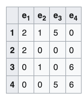
Incidence matrixPermalink

• A V x E matrix, each column encode the (weighted) edge connecting 2 vertices

  

  

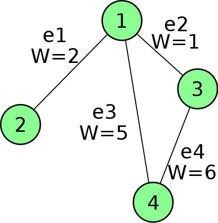
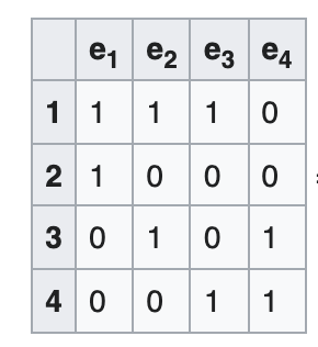
• Sounds familiar? A Jacobian is E x V, each row encodes a measurement connecting 2 variables

  

  

There are even more similarities.

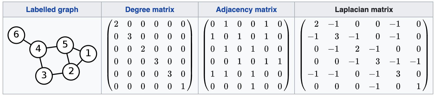
Laplacian matrixPermalink

• Laplacian is given by $L = D - A$, where D and A are degree and adjacency matrices. It is a V x V matrix.
• Graph laplacian depicts the graph’s intrinsic connectivity at the vertices’ perspective.

• Another derivation is $L = MM^\top$, where $M$ is the incidence matrix.

  

• Sounds familiar again? A Fisher Information Matrix is given by $\Lambda = J^\top J$, where $J$ is the Jacobian matrix.
• We will revisit some special setups where $\Lambda$ and $L$ can be directly connected with equations.

Conectivity from LaplacianPermalink

• Key message: we can obtain global topology (graph **connectivity) of the graph via the Laplacian matrix.
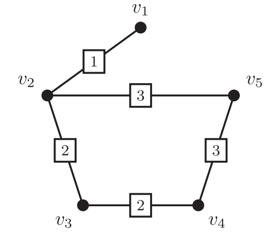
• Measurement 1: Algebraic connectivity / Fielder value
  • $\lambda_2(L)$, where $0 = \lambda_1 \le \cdots \le \lambda_n$
  • This connecivity is 0 if the graph is disconnected; 1 if the graph is complete.
  • For the example above the eigen values are:
    • [3.33066907e-16, 7.21586391e-01, 1.68256939e+00, 3.00000000e+00, 3.70462437e+00, 4.89121985e+00]
  • Associated eigenvector:
    • [0.41486979, 0.30944167, 0.0692328 , -0.22093352, 0.22093352, -0.79354426]
• Measurement 2: Tree connectivity / Kirchoff’s matrix-tree theorem
  • Count the number of spanning trees
    • $$t(G) = \frac{1}{n} \lambda_2 \lambda_3 \cdots\lambda_n$$
    • For the example above: 11
    • Proof: http://math.fau.edu/locke/Graphmat.htm
  • Related: Cayley’s formula $t(G) = n^{n-2}$ for a complete graph.

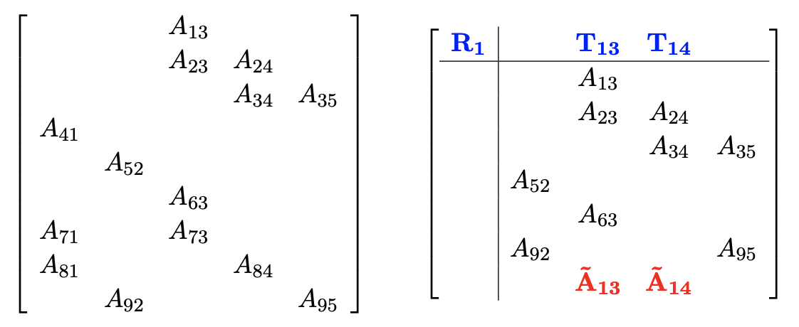
Reduced LaplacianPermalink

• Remove one selected row (vertex) and the corresponding arbitrary column (edge)
• ‘Corresponding to’ a Jacobian: remove a vertex or anchor a variable
• Algebraic connectivity: $\lambda_1(L^r)$
  • SVD / Eigenvalue decomposition
• Tree connectivity: $\det L^r$
  • Relatively easy to compute, esp. for sparse matrices:
    • Use Cholesky decomposition, then compute the product of diagonal elements

Associate Laplacian with InformationPermalink

• The simplest $R^d$-sync problem
  • We have variables $x_j \in \mathbb{R}^d$ and measurements $z_{ij} = x_i - x_j + \epsilon_{ij}$.
  • Covariance per edge is simplified to $\sigma_{i}^2 \mathbf{I}_d$
  • The Jacobian is the incidence matrix (transpose), if d=1 and the variance per edge is 1 and we discard priors

  

• If we take in one prior then the Jacobian is the reduced incident matrix (transpose)

  $$z = \mathbf{M}^{r, \top} x + \epsilon$$

• If we extend to arbitrary dimension d then it becomes

  $z = (\mathbf{M}^r \otimes \mathbf{I}_d)^\top x + \epsilon$ (Kronecker multipler expands each 1x1 entry to a dxd block)

• Then considering the variance as a diagonal weight matrix, the information matrix is given by

  $$\Lambda = (\mathbf{M}^r \otimes \mathbf{I}_d)^\top (\mathbf{W} \otimes \mathbf{I}_d) (\mathbf{M}^r \otimes \mathbf{I}_d) = (\mathbf{M}^r \mathbf{W} \mathbf{M}^r)^\top \otimes \mathbf{I}_d = \mathbf{L}^r_w \otimes \mathbf{I}_d$$

  Here we are using the weighted Laplacian, where the weight per edge is given by the measurement variance.

• This is a very close association between Information and Laplacian matrices.

  $$\Lambda = \mathbf{L}^r_w \otimes \mathbf{I}_d$$

E-Optimal and Albegraic connectivityPermalink

• Covariance is inverse information $\mathbf{C}^{-1} \approx \Lambda = \mathbf{L}^r_w \otimes \mathbf{I}_d$
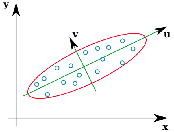
• If we apply eigenvalue decomposition to a covariance matrix C, then the max eigenvalue gives the worst case error variance (E-optimal design) among all unit directions.
• $$\lambda_{max}(C) \approx 1 / \lambda_1(\Lambda) = 1 / \lambda_1(L_w^r)$$

• So the albebraic connectivity defines the variance error bound

  

D-criterion and Tree connectivityPermalink

• If we apply determinant to a covariance matrix C, then the value provides a scalar measure of the uncertainty (D-criterion) in the covariance matrix.
• $$\log \det C \approx \log \det \Lambda^{-1} = - \log \det (\mathbf{L}^r_w \otimes \mathbf{I}_d) = -d \log t(G)$$
• So the tree connectivity gives the uncertainty estimate

There are extensions to less trivial 2D/3D SLAM, and corresponding corollaries. In a nutshell, graph topology and estimation uncertainty is connected via Laplacian and Fisher Information.

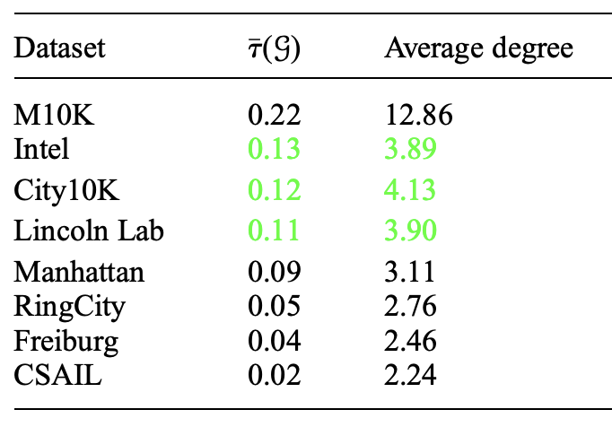
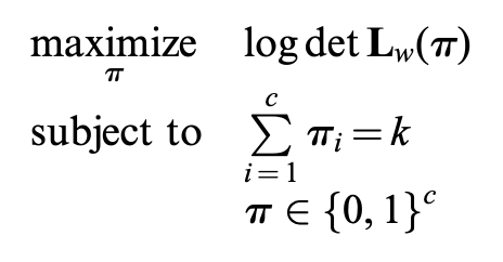
Topology selection for a better D-criterionPermalink

With the empirical connection, we drop covariance now and consider only the topology or the Laplacian

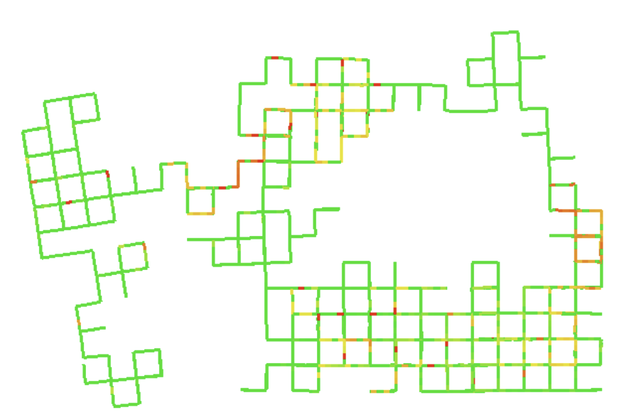
We are interested in edge selection (e.g., loop closure selection in a pose graph)

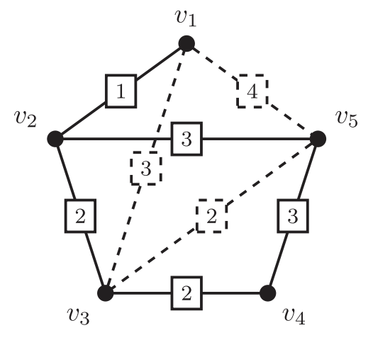
• k-ESP: Given a initial graph and several candidate edges (say potential loop closures), select at most k-edges to maximize connectivity and reduce uncertainty
• $\Delta$-ESP: Select as few edges as possible to reach the desired information gain $\Delta$

We know this can be computed in a batch:

• Select several edges, run Cholesky of the updated Laplacian, and measure t(G) (tree connectivity)
• Exact solution by evaluating in a batches is NP-hard. There are C(m, k) combinations.

Can we do it incrementally by adding one edge $m_e$ in the incidence matrix?

• Yes, the gain is given by $\Delta_e = m_e^\top L^{-1} m_e$, where $m_e$ is the additional column in the incidence matrix

• So we can use the greedy algorithm: every time we add the edge with the max gain, then update the Laplacian

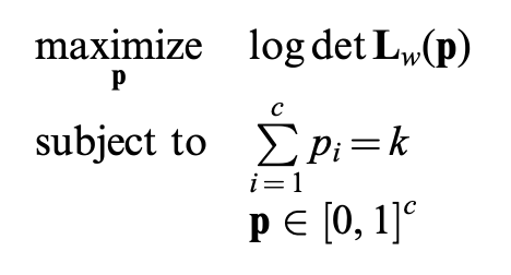
• Other solutions include convex relaxation

  $$L = L_{init} + \sum_j \pi_j L_{e_j} = MW^\pi M$$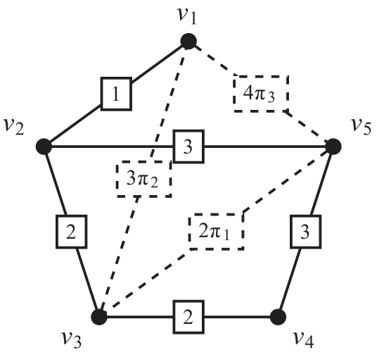

  

• Non-convex version

  

• Convex relaxation (can be solved with a laplacian multiplier

  

• In short: we know a criteria to properly select edges (loops) by (weighted) topology.

ProblemsPermalink

• Can we generalize from the block diagonal covariance to general covariance? In other words, can we put more information to edges rather than a scalar weight?
• Can we put noisy-or factors on edges to support multi-hypothesis inference?
• Tree-connectivity is a global measurement. Can we limit it in a subgraph and consider properties in clique trees?
  • For a clique we can use Cayley’s formula to directly obtain tree connectivity without decomposition. can this help in connectivity measurement?